What's your Relationship Type? How Cardinality Helps Agents to Merge Tables

TLDR: When semantically merging tables using AI agents, specifying a relationship_type (one-to-one, one-to-many, many-to-one, or many-to-many) enables the right collation of data and make clash detection and resolution possible. We show how merging tables with any cardinality becomes very simple with the everyrow SDK and give examples for each of the four relationship types. Table order matters a lot due to the implementation of the agent-based merging.

Why Cardinality Matters

In our previous article, we demonstrated how a progressive approach to semantic table merging achieves high accuracy without any fine-tuning or parameter adaption. However, in some examples we saw high false positive rates as the agent was too confident before collecting evidence and matched, e.g., several CEOs to the same company. The individual match looked plausible to the LLM, but violated a constraint that any human would enforce: a CEO leads exactly one company at a time.

This is where cardinality constraints can help. By declaring the relationship type upfront, the merge system can:

1. Detect clashes: identify cases where multiple left rows matched the same right row (or vice versa)
2. Re-run them with more effort: escalate clashed rows to web-verified matching for higher confidence
3. Mark truly ambiguous cases as unmatched: rather than guessing, leave them for human review

When Do These Relationship Types Arise?

In database theory, the cardinality of a relationship describes how many records on one side can relate to records on the other. Every data practitioner learns this early: a customer has many orders, but each order belongs to exactly one customer. It is one of the first things you define when designing a database schema. In practice, you often have two or more datasets where the relationship of the data and the cardinality is obvious to you, however, the datasets do not have or do not share keys or identifiers. Either you want to match an entity from one table with the same entity in the other table, or you want to match different entities with each other and know how they relate to each other. This is where you can use semantic table merging using AI agents. There are also examples beyond merging datasets: for example, you want to map given data to a set of categories, taxonomies, or properties. Or you want to cluster data based on a certain similarity.

The relationship_type Parameter

In the everyrow SDK that we introduced last time, merging tables semantically with a specific cardinality is now straightforward, by using the new relationship_type parameter:

from everyrow.ops import merge

result = await merge(
    task="<describe the relationship / matching criteria>",
    left_table=...,
    right_table=...,
    relationship_type="many_to_one"  # (default) / "one_to_one" / "one_to_many" / "many_to_many" --> enforce cardinality
)
print(result.data.head)

If there are several matches in the "one_to_many" and the "many_to_many" case, the results are concatenated with " | ". If several rows from the left table point to the same row in the right table for "many_to_one" or "one_to_one", clash resolution is performed: the merge algorithm is run again on all unmatched rows and the rows involved in the clashes, forcing the agents to use web search to first collect evidence before trying to match them again. If clashes persist after the re-run, the affected rows are marked as unmatched rather than forced into an incorrect match.

Let's see how this works on real examples.

1. One-to-One: Company to CEO

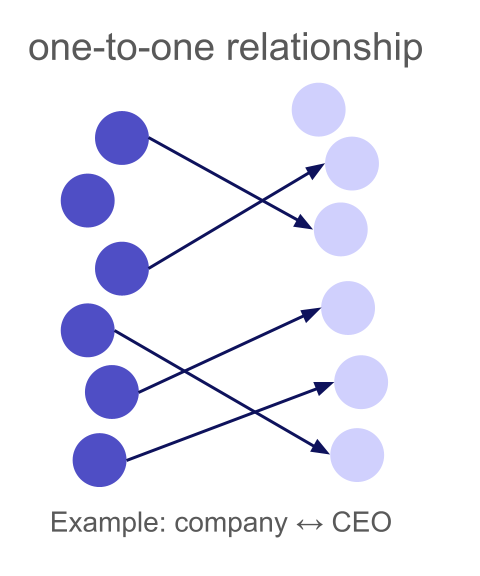
A one-to-one relationship means each left row matches at most one right row, and each right row matches at most one left row. This is the most constrained type: a bijection between matched subsets.

To illustrate this, let us look again at our example (Experiment 3) from the previous article where we merged 438 companies to their CEOs (we implicitely used a many-to-one relationship type). The LLM (Gemini-3-Flash low reasoning, which is our default model for merge) did well on well-known executives (like Tim Cook and Satya Nadella), but for less famous CEOs, it sometimes assigned the same person to multiple companies. In total, it only had an accuracy of 87.3% with 12.3% false positives.

Now let us add the one-to-one constraint to the same table merge:

left_table = data.drop(columns=["CEO"])
right_table = data[["CEO"]]

result = await merge(
    task="Merge the CEO to the company information, use web search if unsure",
    left_table=left_table,
    right_table=right_table,
    relationship_type="one_to_one"
)

The difference is striking. With one_to_one, clashed rows are re-run with web verification. Some genuinely ambiguous cases are left unmatched (the X% drop in match rate), but false positives drop from 12.3% to just Y%, a 9x reduction.

The slight cost increase ($3.97 to$4.81) comes from web search re-runs on clashed rows. This is a worthwhile trade: you're paying ~$0.84 extra to eliminate almost all false positives from a 438-row merge.

2. Many-to-One: Drugs and Paper Authors

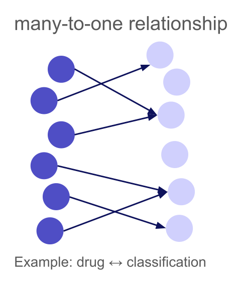
A many-to-one relationship means multiple left rows can match the same right row, but each left row matches at most one right row. This is common when mapping entities to categories, taxonomies, or finding the "parent" of each item.

Drugs to Classifications: When the LLM Already Knows

A natural many-to-one example is mapping entities to a fixed taxonomy. We have 100 common drugs and 39 ATC (Anatomical Therapeutic Chemical) classifications:

This is a textbook many-to-one: multiple drugs share the same classification (Ibuprofen, Naproxen, and Diclofenac are all NSAIDs), but each drug has exactly one primary ATC classification.

result = await merge(
    task="Find the ATC classification of each drug",
    left_table=drugs_df,
    right_table=classifications_df,
    relationship_type="many_to_one",
)

This works beautifully. Drug classifications are well-established medical knowledge, deeply embedded in LLM training data. The LLM matches all of drugs directly, no need for websearch. The many_to_one constraint is important here: it tells the system that it's perfectly fine for multiple drugs to map to "NSAID" or "Opioid analgesic". Without this, the system might flag these shared mappings as clashes and waste time re-running them.

Looking at the false positives, these were really edge cases, like Sotalol → "Beta blocker" instead of "Class III antiarrhythmic", one of the very few drugs that actually has two classifications because it is used to treat multiple conditions.

Papers to First Authors: When Web Search Helps

Not all many-to-one merges are this straightforward. Consider matching research papers to their first (main) author from a list of researchers. Each paper has exactly one first author, but a researcher is typically the first author on several papers in our dataset — a classic many-to-one relationship.

result = await merge(
    task="Merge first authors to research papers",
    left_table=papers_df,      # 895 papers
    right_table=authors_df,    # 303 researchers
    relationship_type="many_to_one",
)

Unlike drug classification, the LLM doesn't inherently know who authored which paper, unless it is a very famous one. But the many-to-one direction (paper → author) makes the web agent's job tractable: a paper's author list is typically right there on its abstract page. Finding the first author is a straightforward lookup. Even for obscure papers outside the LLM's training data, a single web search for the paper title reveals the author list immediately.

3. One-to-Many: Why Direction Matters

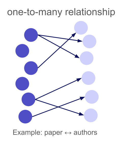
A one-to-many relationship means each left row can match multiple right rows, but each right row matches at most one left row. The "one" side is the left table, the "many" side is the right.

"Isn't one-to-many just many-to-one with the tables swapped?" Technically, yes — but table order matters enormously for agent-based merging, depending on your merge-strategy and implementation. Wrong direction can tank both accuracy and cost.

The everyrow merge strategy processes one left row at a time. For each left row, it shows the LLM (or web agent) that single row alongside the entire right table (or a batch of it if the table is too large) and asks: "which right row(s) match?" The web agent also researches the left row specifically, looking up information to help disambiguate. Of course, this is a design choice: in principle you could enrich also the right table with additional web-research from the web. However, we found that there are almost no cases where this is actually necessary.

This means:

• The left table should contain the entities you want to research individually
• The right table should contain the candidates you're matching against

But there are more reasons why table order matters. In our setup, where we match one entity from the left table with the right table, it is basically a "needle in the haystack" problem: the LLM has to pay attention to all entities of the right table at once and find the right pattern in it. And of course this works better, if the "haystack" is rather small. So if you for example match a huge table of 5000 drugs to just 50 classifications, it is very easy for the LLM to find the right classification for each drug. But when you look for all drugs for a specific classification, always has to split its attention to all drugs at once and pick the right ones. In the end this is a trade-off between number of agents and context length:

• left table large, right table small: many agents but little context per agent
• left table small, right table large: few agents but lots of context per agent So depending on how hard the matching is, to utilize more agents to trade accuracy for resources.

The Paper-Author Problem, Reversed

To illustrate why direction matters, let's reverse the paper-author merge from Chapter 2. Instead of "find the first author of this paper" (many_to_one), we now ask "find all first-authored papers of this researcher from this list" (one_to_many).

The everyrow command is straight-forward, we just have to swap the dataframes, swap the relationship type and adapt the prompt:

# Reversed: researchers on the left, papers on the right
result = await merge(
    task="Merge first authors papers to researchers",
    left_table=authors_df,    # 303 researchers
    right_table=papers_df,    # 895 papers
    relationship_type="one_to_many",
)

However, the results now look quite different:

The reversed configuration is worse on every metric. Why? Because finding "which papers did this researcher first-author?" is fundamentally harder than "who is the first author of this paper?" A paper's author list is right there on the abstract page — one web search, one answer. But a prolific researcher may have published hundreds of papers, and the agent has to figure out which specific papers from our list of 895 they were the first author on. That requires navigating Google Scholar profiles, university pages, or DBLP, and then cross-referencing against a long list of candidate papers.

Products to Reviews: A Natural One-to-Many

Where one-to-many truly shines is when the "one" side contains well-defined, searchable entities and the "many" side contains noisy, unidentifiable items. Consider matching products to their customer reviews:

Each product has multiple reviews, but each review is about exactly one product — a natural one-to-many relationship.

result = await merge(
    task="Find the reviews for this product",
    left_table=products_df,    # 50 products
    right_table=reviews_df,    # 98 reviews
    relationship_type="one_to_many",
)

The table order works perfectly here. Products like "Apple AirPods Pro" or "Sony WH-1000XM5" are well-defined entities the agent can reason about — their features, specs, and characteristics are well-known. Reviews, on the other hand, are anonymous snippets like "Excellent battery. Last me around 6 hours of play time" — you can't meaningfully search the web for a review, and a review on its own is a noisy, unidentifiable piece of text. Putting the identifiable products on the left gives the agent something concrete to work with when matching.

Reversing this merge (reviews on the left, products on the right, many_to_one) would force the agent to start from each anonymous review and try to figure out which product it's about — a much harder task without the product context to guide the matching.

Rule of thumb: put the entity that is easier to research individually on the left, and the reference set on the right. This applies to both many-to-one and one-to-many merges.

4. Many-to-Many: Companies and Investors

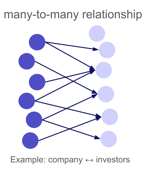
A many-to-many relationship is the most general case: any left row can match multiple right rows, and any right row can match multiple left rows. There are no uniqueness constraints at all.

Example: Companies and their investors. A company has multiple investors, and an investor holds stakes in multiple companies. Vanguard is a top shareholder in hundreds of S&P 500 companies, and Apple has dozens of institutional investors.

We have 49 companies (from tech giants to private startups) and 65 investors (institutional asset managers, venture capital firms, and corporate investors):

Here the table ordering matters for a different reason. We put companies on the left because a company typically has fewer investors (3-10 major ones) than an investor has portfolio companies (potentially hundreds). This means the web agent's task, "find the major investors of Adobe," is more tractable than "list all companies Vanguard invests in."

result = await merge(
    task="Find all investors of each company",
    left_table=companies_df,
    right_table=investors_df,
    relationship_type="many_to_many",
    merge_model="gemini-3-flash-thinking",
    use_web_search="yes",
)

Many-to-many is the hardest relationship type. The system cannot use clash detection (any match pattern is theoretically valid), so it relies entirely on the quality of individual match decisions. Web search is critical here: 61.8% of matches required web verification. For private companies like Anthropic, Canva, Databricks, and Klarna, investor information is often not in LLM training data, making web search essential.

The 4.8% false positive rate reflects the inherent difficulty: investor relationships change frequently (funds rebalance, companies go through funding rounds), and the boundary between "major investor" and "minor stake" is fuzzy. Despite this, the merge captures the major institutional holders accurately for most public companies.

Summary: Choosing the Right Cardinality

The key insight is that cardinality is not just a schema annotation, it's a constraint that helps the system produce better results. By detecting and resolving clashes, one-to-one and one-to-many merges achieve significantly lower false positive rates. And by choosing the right table order for many-to-one and many-to-many, you make the web agents' job easier, improving both accuracy and cost.

Try It Yourself

The relationship_type parameter is available in the everyrow SDK. Install it and try on your own data:

pip install everyrow

from everyrow.ops import merge

result = await merge(
    task="Describe your merge task here",
    left_table=your_left_df,
    right_table=your_right_df,
    relationship_type="one_to_one",  # or "one_to_many", "many_to_one", "many_to_many"
)

The output includes a research column with justifications for each match, so you can audit the reasoning. Check the SDK documentation for full API details and more examples.

Pro tip: You can now use everyrow easily in Claude Code, using the everyrow-mcp: First, add this to your mcp json or settings:

{
  "mcpServers": {
    "everyrow": {
      "command": "uvx",
      "args": ["everyrow-mcp"],
      "env": {
        "EVERYROW_API_KEY": "YOUR_EVERYROW_API_KEY"
      }
    }
  }
}

Then you can just upload your csv and tell Claude Code in natural langauge what you want, and it will figure out the best parameters for you.